I’ve been doing archery for a year now, and I’ve slowly worked my way up the ranks. I’m currently ranked 573 out of 1339, give or take, internationally in the Grand Archery Tournament. Locally I’m 39 out of 60. Or I was… I may have just jumped to 30th place because Sunday was insane.

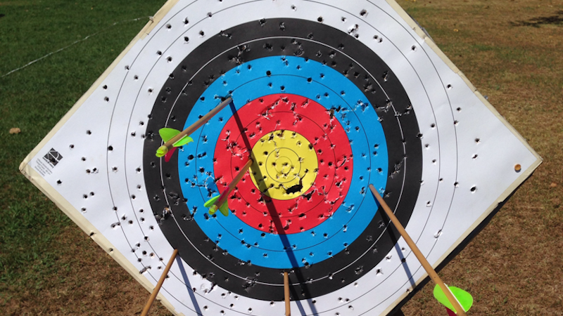
Yellow is 5 points, white is 1. That right there is 16 points (the arrow in the lower middle actually broke the line and was in the blue for 3 points, it fell after the arrow someone else shot below it was moved). Now, you’re thinking “16, so? With six arrows, you can get 30!” This is true. But my previous record at that distance was 7. That would be an improvement.
I ended up shooting a 55 for the day, and just to explain, the highest score of the day was a 75 (I think), by Hugh, who is on his way to becoming the best shot in the land. The way we rank ourselves is easy. 0-24 average is a Novice, 25-44 is Bowman, 45-64 is Yeoman, 65-84 is Forrester, and 85-104 is Bowmaster. If you get over 105, you’re a Royal Bowmaster. We have two Bowmasters, and no Royals. I made Bowman in May, which was my personal goal, and I’ve kept my score above that.
Oh, you know I’m a nerd, right?

I have a spreadsheet in Numbers where I put in the date and my score for each round. The Averages for the yards and arrows are a basic Average query. I don’t know why we track how many arrows we can shoot in a speed end (30 seconds) but we do. So that’s my basic record, and at a glance it’s pretty nice. The jump from 11 to 25 happened when I got my own bow, and I started hitting the 30s once I got my new glasses. May 4th is when I made Bowman officially.
But that’s not all I do with my stats. You see, I also have this:
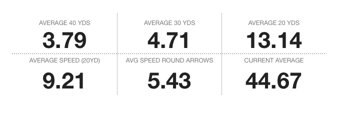
I know, that’s a little weird. I made a second ‘table’ on the spreadsheet for this. The first table is called “Scores” and this one is called “Averages” and these are the basic averages for each distance. They are exactly the math you think they are: =AVERAGE(Scores::B)
It’s all very basic until you hit “Current Average”, which is not actually my true average. It’s my SCA average, which is the highest 3 scores: =AVERAGE(LARGE(Scores::G,1),LARGE(Scores::G,2),LARGE(Scores::G,3))
I’m using the LARGE() function to grab the highest 3 in this way, because the AVERAGE() function is a bit of a pill. But this is wrong as well as inefficient. We actually only check the highest 3 scores in the last 12 months, which makes my math this: =AVERAGEIFS(Scores::G,Scores::A,">=" & (TODAY()−365),Scores::G,">=" & LARGE(Scores::G,3) )
It took me a long time to figure that out. I’m not very good with Excel/Numbers.
Finally we have my last table, “Chart.”

This is soooo fun. It’s just a simple trendline chart. Values (left) are the scores. Names (bottom) are the dates. I set the trendline to be the Moving Average, so the bars show you my scores and the blue line shows you the average and how it’s gone up and down a little.
What kills me a little is my average right now is 44.67. A 45 is Yeoman! We don’t round up! KHAAAAAAAAAAAAAAAAN!